Fraud detection sounds like a solved problem until you look at the data. The core issue is not building a classifier. It is building one that works when 99.8% of the data belongs to one class and 0.2% belongs to the other. A model that always predicts "legitimate" gets 99.8% accuracy. It also catches zero fraud. That is the whole problem in one sentence.
Most tutorials on this dataset immediately reach for SMOTE or random oversampling to balance the classes before training. I wanted to take a different approach. What happens when you throw standard ML models at a real imbalanced dataset and refuse to artificially balance it? No SMOTE. No undersampling. Just raw class imbalance, three models, and honest evaluation.
The dataset contains 284,807 credit card transactions made by European cardholders over two days in September 2013. Of those, 492 are fraudulent. That is 0.172%. For every fraud in the data, there are roughly 578 legitimate purchases. This is not a textbook 50/50 split. This is the real distribution that production systems face, and I wanted to see how far off-the-shelf models could get without synthetic tricks.
Card fraud costs the global economy billions annually. But the dollar figures matter less than the shape of the problem: rare events buried in massive volumes of normal activity. Catching them requires models that pay attention to the 0.172%, not the 99.828%.
Financial institutions walk a narrow line between two failures. Let fraud through, and you absorb direct losses plus investigation costs. Flag too many legitimate transactions, and you frustrate customers who take their business elsewhere. The classifier has to be precise in both directions.
The data comes from a research collaboration between ULB (Universite Libre de Bruxelles) and Worldline, one of Europe's largest payment processors. It captures two consecutive days of card-present and card-not-present transactions across the European market. The dataset is publicly available on Kaggle and is one of the most commonly used benchmarks for imbalanced classification research.
There are 30 input features and one binary target variable (Class: 0 for legitimate, 1 for fraud).
Twenty-eight of those features, V1 through V28, are PCA-transformed. The original attributes were stripped for cardholder privacy, which is standard in financial datasets. You cannot reverse-engineer the original feature names from PCA components, but the statistical relationships between variables are fully preserved. That is the whole point of PCA in this context: protect the data while keeping the signal intact.
The remaining two features are provided in their original form. Time measures seconds elapsed since the first transaction in the dataset, spanning roughly 48 hours (0 to 172,792 seconds). Amount is the transaction value in euros, ranging from 0.00 to 25,691.16 across the full dataset.
There are no missing values anywhere, which eliminated the need for any imputation strategy. The class split: 284,315 legitimate and 492 fraudulent. That is a 578:1 imbalance ratio, firmly in the "extreme imbalance" territory where standard approaches start to break down.
Fraudulent transaction amounts max out at 2,125.87 euros, while legitimate transactions go as high as 25,691.16. That ceiling difference is telling. Fraudsters tend to stay below thresholds that trigger automatic holds.
Before training anything, I spent time looking at the data. EDA is where you build intuition about what the models will find easy and what they will struggle with.
Four PCA features stood out as the strongest fraud indicators: V17, V12, V14, and V10. All four show strong negative correlations with the fraud label. When these features take lower values, the probability of fraud increases. The consistency of the negative direction across all four suggests PCA captured a coherent fraud dimension in the data. These features are doing most of the work.
On the other end, features like V25, V26, and V28 show almost no correlation with fraud. Their distributions look identical across both classes. Since PCA components are orthogonal by construction, keeping them does not introduce multicollinearity. But they contribute close to zero discriminative power. The models would naturally ignore them, and they did.
For the top features, kernel density plots show clean class separation. V14 is the most visually obvious: the legitimate class is roughly normal around zero, while the fraudulent class shifts hard to the left with almost no overlap. That kind of separation in feature space is exactly what classifiers exploit, and it explains why even a simple linear model can get surprisingly far on this task.
Transaction amounts told an interesting story. Fraudulent transactions have a higher mean ($122) but a lower median ($9.25) compared to legitimate ones (mean ~$88, median ~$22). That gap between mean and median points to a bimodal fraud strategy.
The low median reflects small test charges, typically $1 to $10, that fraudsters use to verify a stolen card is active. The elevated mean reflects the larger extraction attempts that follow. The result is a distribution with higher variance than normal consumer spending. Fraudsters probe both ends of the amount spectrum.
Time patterns were subtler but consistent. Transaction volume follows the expected diurnal cycle: peaks during the day, drops at night. The two-day capture window produces two clear humps in the distribution, one per day. Fraudulent transactions do not follow this cycle as closely. The fraud-to-legitimate ratio ticks up during low-volume overnight hours.
This makes sense operationally. Fewer transactions means fewer concurrent alerts. Monitoring teams may have fewer analysts on overnight shifts. Cardholders are asleep and not checking their statements in real time. By the time anyone notices, the fraudster has moved on. Higher amounts and lower time values both correlate with fraud, though the time signal is weaker than the PCA features.
The Time and Amount features were standardized with scikit-learn's StandardScaler to zero mean and unit variance. Without scaling, Amount values ranging into the thousands would dominate distance-based calculations and gradient updates. Time values in the hundreds of thousands would create numerical issues.
The 28 PCA features were already scaled by the PCA transform itself, so I left them alone. No additional feature engineering was needed. The PCA components are orthogonal and normalized by construction.
I compared 70/30 and 80/20 train-test splits. Both used stratified sampling to maintain the 0.172% fraud rate in each set. The size increase from 70/30 to 80/20 did not produce a meaningful improvement in any model. The models had enough data either way. The bottleneck was the imbalance, not the training set size.
I deliberately did not apply any resampling technique. No SMOTE, no random oversampling, no undersampling. The class imbalance was preserved as-is throughout training and evaluation. I wanted to see what the models could actually learn from the real distribution. If the signal is strong enough in V17, V12, V14, and V10, the models should find it without artificial help. That was the bet.
The reasoning: resampling changes the data distribution your model learns from. SMOTE generates synthetic minority examples by interpolating between existing ones. That can help, but it can also introduce artifacts that do not reflect real fraud patterns. Undersampling throws away 99.8% of your legitimate data, which is a massive information loss. The legitimate class is not homogeneous. It contains diverse spending patterns across different amounts, time periods, and merchant behaviors. Reducing it to a few hundred samples cannot represent that diversity.
I wanted a clean baseline first. Know what the models can do on raw data before deciding whether resampling is worth the tradeoffs.
Linear classifier. Models the log-odds of fraud as a linear combination of input features. I trained it with L2 regularization and balanced class weights, which adjusts the loss function to penalize minority-class errors more heavily in proportion to the imbalance ratio.
The balanced weights are important here. Without them, the model would barely learn what fraud looks like because the gradient signal from 492 fraud examples gets drowned out by 284,315 legitimate ones.
It has one major advantage over the other two models: interpretability. Every feature gets a coefficient you can read, explain, and defend. Positive coefficients push toward fraud, negative toward legitimate. In finance, where auditors and regulators ask why a specific transaction was flagged, that transparency is not optional. You need to be able to say "this transaction was flagged because V14 was unusually low and the amount was higher than normal."
It reached 99.93% accuracy. Decent precision, but limited by its linear decision boundary. Some fraud patterns in this data involve interactions between features that a straight line through feature space cannot separate. The model works well as a baseline. It tells you the floor. But it leaves room on the table for non-linear methods.
Non-linear by design. Splits the feature space into rectangular regions through a sequence of binary decisions on individual features, picking each split to maximize information gain (minimize Gini impurity). It captures interactions between features without any manual feature engineering, which is a real improvement over the linear model.
The tradeoff is stability. Single trees overfit. Small changes in training data can produce a completely different tree structure, which means different predictions on the same inputs. I constrained tree depth and minimum samples per leaf to reduce this tendency, but it is inherent to the algorithm.
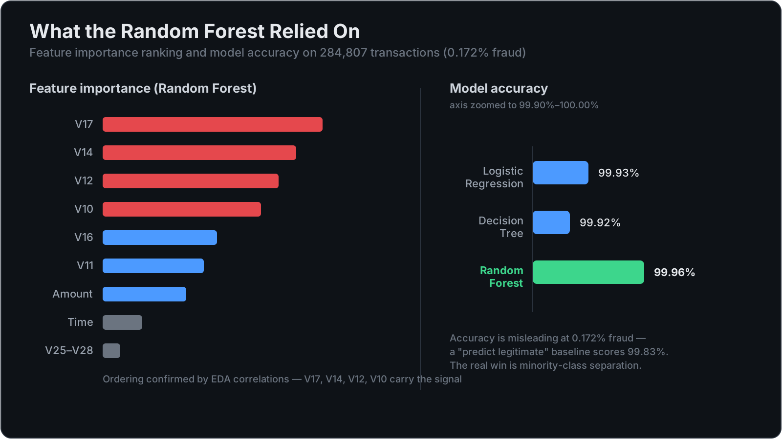
It hit 99.92% accuracy. It also provided a natural feature importance ranking based on how much each feature reduces impurity across its splits. The ranking matched the correlation analysis from EDA: V17, V12, V14, and V10 at the top. The tree essentially rediscovered the same fraud signals through a completely different method, which gave me confidence those features were genuinely informative and not statistical noise.
An ensemble of 200 decision trees trained on bootstrapped subsets of the data. Each tree sees a random subset of features at each split, which forces diversity across the ensemble. Final predictions come from majority voting across all 200 trees.
The bootstrap sampling and feature randomization together solve the variance problem that makes single trees unreliable. Any single tree might overfit to quirks in its training subset. But when you average predictions across 200 trees, each trained on different data with different feature subsets, the quirks cancel out and the real signal survives.
The result is a model that is both more accurate and more stable than any individual tree. It also produces a more trustworthy feature importance ranking, since importance is averaged across 200 independent views of the data rather than depending on the structure of one particular tree.
Random Forest reached 99.96% accuracy with the best precision and recall of the three models. The 200-tree ensemble pays for itself in stability and performance. Training takes longer, but at inference time each tree can predict independently, so it parallelizes well.
| Model | Accuracy |
|---|
| Logistic Regression | 99.93% |
| Decision Tree | 99.92% |
| Random Forest | 99.96% |
Random Forest wins across the board. But those accuracy numbers deserve skepticism.
When your dataset is 99.828% one class, accuracy is almost meaningless. A model that predicts "legitimate" for every single input gets 99.828% accuracy. It has learned nothing. It catches zero fraud. On this dataset, that naive model would let all 492 fraudulent transactions pass through unchallenged.
The real story is in minority class performance. How well does each model separate the 492 fraud cases from the 284,315 legitimate ones? Random Forest produced the best separation. Logistic Regression struggled with non-linear fraud patterns. Decision Tree captured those patterns but was noisy and unstable about it. Random Forest smoothed out that noise across 200 trees and delivered the most reliable predictions.
The difference between 99.92% and 99.96% looks tiny in percentage terms. In absolute terms, on 284,807 transactions, that gap represents real fraudulent transactions correctly caught or missed. Each one could mean hundreds of dollars. Scale that to a real payment processor handling millions of transactions per day, and small differences in model performance translate into significant dollar amounts.
Going from the 70/30 split to 80/20 did not meaningfully change these numbers. The models were not data-starved. The challenge was always the imbalance, not the volume. Adding more training data did not help because the problem was never about having too little data. It was about having 578 times more of one class than the other.
In a production system, you would not stop at accuracy. You would tune the classification threshold based on business costs. Lowering the threshold catches more fraud (higher recall) but flags more legitimate transactions (lower precision). Raising it does the opposite.
The right threshold depends on what a missed fraud costs versus what a false alarm costs. That is a business decision, not a modeling decision. The model provides calibrated probabilities. Where you draw the line is up to the fraud team. A bank processing millions of transactions per day cannot manually review every flagged transaction. The threshold has to produce a manageable alert volume.
The feature importance ranking from Random Forest confirmed everything the EDA suggested. V17 is the single most important feature. V14, V12, and V10 follow. Those four carry a disproportionate share of the model's discriminative power. The Amount feature sits in the middle tier. Time is near the bottom. The low-information PCA features (V25, V26, V28) contribute almost nothing, as expected.
The biggest takeaway is that accuracy is a trap in imbalanced classification. You can get 99%+ accuracy by doing literally nothing useful. The metrics that matter are precision, recall, and AUC-ROC. If your fraud detector has high accuracy but low recall, it is missing the frauds that actually cost money. I will never look at a 99% accuracy claim the same way again without asking "what is the class distribution?"
Working without resampling was a deliberate choice and I am glad I made it. It forced me to confront what the models could actually learn from the raw data distribution. The results were strong enough to question whether resampling is always necessary. Sometimes the signal is there, even at 0.172%. V17, V12, V14, and V10 carry enough information to separate the classes without synthetic help.
The EDA phase was more valuable than I expected. Looking at distributions and correlations before training built intuition that made the model results make sense instead of being black-box numbers. When Random Forest flagged V17 as the most important feature, I already knew why. That kind of understanding matters when you need to explain your model to someone who is not a data scientist.
Knowing which features matter is useful beyond model training. If you are building a monitoring dashboard, you focus on V17 and V14. If you are deploying a lightweight model at the edge where compute is limited, you can drop the bottom 10 features and lose almost nothing. Feature importance is not just a model diagnostic. It is operational intelligence.
Ensemble methods earn their complexity. The jump from a single Decision Tree to a 200-tree Random Forest was the single biggest improvement in this project. Variance reduction through averaging is not a theoretical nicety. It showed up directly in every metric. More trees, more stability, better results.
I started with 100 trees and moved to 200. The improvement from 100 to 200 was small but measurable. Diminishing returns set in, but 200 was a reasonable sweet spot for this dataset size.
Not applying resampling was the right call for understanding the problem, but I would not recommend it as a universal strategy. On datasets where the minority class signal is weaker or noisier, you might need SMOTE or cost-sensitive learning to get usable recall. This dataset had unusually clean separation in the top PCA features. That will not always be the case.
If I were to extend this, I would look at precision-recall curves for threshold tuning and test gradient boosting methods like XGBoost, which often outperform Random Forest on structured data. I would also evaluate how the models degrade over time as fraud patterns shift.
The dataset is from 2013. Fraud has evolved since then. A model trained on 2013 patterns would drift in production without retraining on fresh data. Concept drift is real, and any production fraud system needs automated monitoring and retraining pipelines to stay effective.
I would also explore SHAP values for individual prediction explanations. Knowing that V17 is important globally is one thing. Being able to explain why a specific transaction was flagged is a different and harder problem. In regulated environments, that per-prediction explainability is a compliance requirement, not a nice-to-have.
Python for everything. pandas and NumPy for data manipulation. scikit-learn for all three models and preprocessing (StandardScaler, train_test_split, classification metrics). Matplotlib and Seaborn for visualization during EDA. Jupyter Notebook as the development environment. The entire pipeline runs in a single notebook, from data loading through evaluation.